Probabilistically Counting the Districtings of a Graph

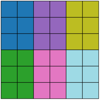
Given a planar graph \(G = (V,E)\) and district sizes \(\lbrace k_i\rbrace_{i=1}^n\), a political districting of \(G = (V,E)\) is a partition \(\lbrace P_i\rbrace_{i=1}^n\) of \(G\) into (simply-)connected subgraphs (called districts) satisfying \(|P_i|=k_i\).

For the purposes of this project, I’ve usually taken \(G\) be an \(n\times n\) grid graph and \(k_i=n\) for all \(i\); but this was a choice made of convenience, not necessity. This project explores a method to stochastically estimate the number of districtings of \(G\) when enumerating them is not computationally viable.

An Analogy.

Here’s an analogy for how this chain works: everyday, Gretel’s parents drop her off at a (uniformly) random spot in the Black Forest, until she is able to tell them how many trees there are in the forest. At first, Gretel tried leaving a paint mark on the tree closest to where she was dropped off, and tallying the number \(L\) of days it took for her to run back into a tree she had already marked. She’s able to calculate how many days this would take if the forest had size \(M\); so, by repeating this experiment many times (maybe changing the color of her paint every time she gets a hitting time \(L\)), she will find an estimate of \(L\) that she is confident in, and she can then reverse-engineer an estimate of \(M\) from this value. This describes the main chain of this method.

But Gretel soon realized that \(L\) was way too big – it was taking her too long to run into a tree she had already marked – so she changed her strategy. Now, she hangs up a (relatively loud) wind chime where she gets dropped off every day. She knows that she can hear any of these windchimes as long as she is within \(r=100m\) of it; and she figured out that there are usually \(N_r=1000\) trees within any 100m radius inside the forest. Now she just measures the number of days until she is dropped off in a spot where she can hear one of her wind chimes; by multiplying this number of days by 1000, she gets something akin to the hitting time \(L\) she was previously measuring. The process of estimating the volume \(N_r\) of a metric ball in the forest is what I refer to as the calibration chain.

The Mathematical Outline.

Use the notation \(𝓜_n (G)\) for the space of all districtings of \(G\) into \(n\) districts; we are interested in \(M = |𝓜_n (G)|\). The main idea of this method is to uniformly sample districtings from \(𝓜_n (G)\) until we run into one that is within a (astutely chosen) radius \(r\) of a districting in our past. When that happens, we measure a hitting time \(L\) as the number of states we had visited before hitting, and we reset the past of the chain. For example, the run of the chain below, which was sampling states uniformly from \(\lbrace 1,\ldots,100\rbrace\) with \(r=0\), would have a hitting time of \(L=7\):

\[X_1 = 15, X_2 = 81, X_3 = 91, X_4 = 39, X_5 = 20, X_6 = 45, X_7 = 39.\]

The reason I describe this as a chain, even if \(X_t\) is just sampled uniformly from \(𝓜_n (G)\), is that it is not easy in practice to generate a districting of \(G\) uniformly at random (cf. [1]). To achieve this, I run a Metropolis version of the Simple Random Walk on \(𝓜_n (G)\), and sample a state every time I am confident we have moved \(t_{mix}\) steps away from the previous sample. The proposal I use for this Simple Random Walk on \(𝓜_n (G)\) is a swap step: two districtings are adjacent if you can reach one from the other by swapping the assignment of two vertices in adjacent districts. (There is more nuance to this Metropolis chain, which I’ll skip here).

We can make some simplifying assumptions about the hitting time \(L\) to calculate the expection \(𝔼(L)\):

1. As we run the chain, the metric balls we sample do not frequently overlap significantly, so that we truly are sampling around \(N_r\) districtings at a time.
2. The hitting time \(L\) is big enough to smooth out the irregularities in the volumes \(N_r\) of the balls we sampled. If \(𝔼(L)\) is too small, then the data we get will depend on the specific balls we sampled, as opposed to the average \(N_r\).

With these simplifying assumptions, we can estimate \[𝔼(L)\approx\displaystyle\sum_{t=1}^{\lceil M/N\rceil -1}\frac{\prod_{j=0}^{t-1}(M-jN)}{M^{t+1}}N(t^2+t).\]

If the value of \(N_r\) is known, the above formula gives us a monotone relation between \(𝔼(L)\) and \(M\). If we have good experimental data on \(𝔼(L)\), we can invert it to solve for \(M\). It’s also worth noting that this formula only really depends on the fractional volume \(f=N/M\) of the metric balls; we could re-arrange it as \[𝔼(L)\approx\displaystyle\sum_{t=1}^{\lceil f^{-1}\rceil -1}f(t^2+t)\prod_{j=0}^{t-1}(1-jf).\]

This chain might feel a bit too messy to be true at first, but you can run a toy version of it on the unit square \([0,1]\times[0,1]\); generate \(M\) nodes uniformly at random, pick \(f= 6\cdot 10^{-6}\) with the Euclidean metric, and see for yourself:

import math
import random

#Toy example
#Generate nodes
M_7 = 158753814 #This is the known size of the 7x7 grid metagraph
nodes = []
for i in range(M_7):
    nodes.append((random.random(),random.random()))
print(nodes[0])

#This next bit mimics the main chain
past = set()
L_times = []
#pick r so that a euclidean ball of radius r contains 6*10**(-6) of the area in [0,1]x[0,1]
r = (6*10**(-6)/math.pi)**(1/2)
for j in range(20000):
    new_node = random.choice(nodes)
    for old_node in past:
        if (new_node[0]-old_node[0])**2 + (new_node[1]-old_node[1])**2 < r**2:
            L_times.append(len(past)+1)
            past = set()
            break
    past.add(new_node)
average_L=sum(L_times)/len(L_times)
print(average_L)

#This next bit is how you would estimate M from a known value of L
def expected_T(N,M):
    factor = float(N/M)
    expectation = 0
    for t in range(math.ceil(M/N)):
        expectation+=factor*(t**2+t)
        factor*=(M-t*N)/M
    return(expectation)

def seek_M(L,N):
    b = 2**int(math.log(L,2)+1)
    overshot = 0
    while not overshot:
        if expected_T(N,b)>L:
            overshot = 1
        else: 
            b*=2
    a = int(b/2)
    while b-a !=1:
        c= (b+a)/2
        if expected_T(N,c)>L:
            b=int(c)
        else:
            a=int(c)
    if expected_T(N,a)-L>L-expected_T(N,b) :
        return b
    else:
        return a

print((seek_M(average_L,6*10**(-6)*M_7)-M_7)/M_7) #This gives us the % error of our estimate of M.

The Pencil Metric.

If none of the rest of the project ends up bearing fruit, this is the one idea I’ve had that I know is worthwhile: we can put a metric \(d\) on \(𝓜_n (G)\) by taking \(d(x,y)\) to be the size of the symmetric difference between the cut edges of \(x\) and \(y\).

That is, the cut edges of a districting \(x\) is the set of edges in \(E\) which connect to separate districts \(P_i,P_j\) for \(i\neq j\). It’s easy to believe that a districting is entirely determined by its set of cut edges, as long as you don’t care about how the districts are labeled.

To see that this satisfies the triangle inequality, I like to think of this analogy: to calculate the pencil distance between \(x\) and \(y\), take a map, drawn in pencil, corresponding to \(x\), and start erasing and drawing new boundaries until you get to the map corresponding to \(y\). Tally up the number of times you had to draw or erase a new boundary between precincts (the vertices of \(G\)), and you get the pencil distance between \(x\) and \(y\). To check the triangle inequality, imagine starting from the map of \(x,\) drawing and erasing until you get to \(y,\) and again until you get to \(z\). Clearly it would have taken you at most as much time to go straight from \(x\) to \(z\).

Here’s some code, using partition objects from the GerryChain package for python:

#needs cut_edges to be added to updaters
def pencil_dist(partition1,partition2):
    return len(partition1.cut_edges.difference(partition2.cut_edges))+len(partition2.cut_edges.difference(partition1.cut_edges))

As discussed above, we want to pick the metric radius \(r\) of the balls we sample to be big enough to reduce our hitting time \(L\) to something computationally manageable, but small enough that our results are still able to give a meaningful estimate of \(M\). In the limit that \(r\) is larger than the diameter of the metagraph, our hitting time \(L\) would be constant \(2\), which could correspond to any value of \(M\). So our estimate of \(M\) loses precision as we increase \(r\).

Heuristically, if the fractional volume \(f\) of our balls is \(\approx 6\cdot 10^{-6}\), we get a hitting time of \(𝔼 L\approx 512\), which is small enough to run computationally, but still big enough to get good precision. The difference between the estimate of \(M\) given by a hitting time of \(L= 512\) and \(L= 513\) is around \(0.3\)% the size of \(M\).

The Calibration Chain.

The goal I had set myself at the beginning of this project was to get an estimate for the size of the 10x10 grid metagraph, which is not currently known (cf. [2]). Currently, the roadblock I am working around is coming up with a way to estimate the volume \(N\) (or fractional volume \(f\)) of metric balls of given radius \(r\) in the metagraph. When \(M\) is small (hence so too is \(N\)), it was possible just to proceed by enumeration: take a metropolis random walk on the metagraph to uniformly sample a partition, then enumerate its neighbors outwards until you’ve travelled a distance \(r\) (there’s some more nuance here too, which I’ll skip).

However, this quickly stops being computationally viable: for the 8x8 graph, we know \(M=187,497,290,034\), so ideally each ball would contain \(6\cdot10^{-6}\cdot M \approx 1,124,983\) states; for reference, the main chain usually samples around \(20,000\) states in total (there’s some nuance here). So we have to design some other stochastic process to estimate \(N\) or \(f\).

My first thought was to run some regressions to see how \(N\) depends on \(r\) for small \(r\), then extrapolate the values of \(N\) we need. This ultimately didn’t work – my estimates of \(M\) were off by around 45% – but I gained some valuable insights from doing this. Notably, it turns out that \(N\) grows exponentially with \(r\) (maybe this is an indication that we could embed the metagraph into a negatively curved space?). For the 8x8 graph, it was viable to enumerate values of \(N\) from \(r=8\) up to \(r=13\); using those 6 datapoints, a linear regression says that

\[N(r) \approx \exp(.64798948r - 1.69862025)\]

My second approach to overcoming this roadblock is to design a chain in two steps:

1. Uniformly sample and store a ‘mesh’ of ~500 partitions from the metagraph;
2. Uniformly sample without storing ~20000 more partitions, and record the number \(X\) of times these fall within a radius \(r\) of one of the mesh states (maybe also recording when the sample is within \(r\) of multiple mesh states).

Assuming minimal overlap (which is reasonable; the main chain tells us that on average it takes ~512 samples to see a sample fall within \(r\) of another), the mesh would cover a fraction \(500\cdot f\) of the state space; so we have an equation

\[500\cdot f \approx X/20000\]

This is basically probabilistic integration of the characteristic function of a metric ball (or 500 such characteristic functions). An analogy here is, if you want to know the area of a dartboard, put 500 of those dartboards on the wall, throw 20000 darts at the wall, average out the number of darts that hit each dartboard, and divide by the number of darts you threw (and then multiply that by the area of the wall, if you want actual volume).

I haven’t actually tried this approach yet in practice! But maybe I’ll get back to it when I have more time for research. It seems like picking the number of mesh states wisely and dealing intelligently with overlaps would be an important consideration.

Results, Applications, and Limitations.

The main positive result I have is from running the main chain on the 7x7 grid metagraph; there, it turns out the appropriate radius to use is \(r=13\); I was able to find that \(N\approx 623.33\) on average by enumeration; and the main chain got a result of \(L\approx 601.52\). This gives an estimate of \(M\approx 143263247\), which is 9% below the known value of \(M=158753814\) – and maybe this precision could be improved with more sampling (I recall one run of the chain gave me a precision of 4%, but that may have been an outlier).

The main appeal of this process is that it is not enumerative; it could theoretically work for the 10x10 grid graph. By picking \(r\) appropriately, you could make the main chain as fast as you like, at the cost of precision.

A secondary appeal is that this chain doesn’t depend at all on the precise geometry of the underlying graph \(G\). If it ran on the 10x10 graph, my next goal would be to run it on Iowa, which has a political map made up of 99 precincts. Or you could also use this chain for other lattices, like the triangular lattice; or you could run it with different district sizes \(k\). You could even run this chain on graphs other than the metagraph \(𝓜\) we’ve been working on.

That being said, a limitation is the metropolis chain that I’m currently running to get uniform sampling of the metagraph. Since this metropolis chain is based on a simple random walk, it requires enumerating all of the swap step neighbors of the current partition in order to pick a neighbor to move to. Worst, swap step proposals move through the metagraph relatively slowly, so the mixing time is high. It seems still feasible to use this uniform sampler for the 10x10 graph; but it’s doubtful that this chain will be usable for most real-world political maps, which can be made up of thousands of precincts.

And another drawback is that ultimately, this isn’t a very interesting question to answer. In the study of structural democracy, we want to do ensemble analysis on the metagraph \(𝓜(G)\) of partitions of a graph; but knowing the size of this metagraph is much less interesting than, for instance, knowing the steady-state distribution of the proposal you’re running, or knowing whether this proposal is irreducible.

This last drawback inspires another (still not very exciting) possible use for the main chain – because the uniform sampler we use to explore the metagraph is based on a swap step chain, the estimate of \(M\) it gives is really an estimate of the size of the connected component of \(𝓜\) it started in. So, in cases where we already know \(M\) from enumerative methods, we could compare the chain’s estimate of \(M\) to the known value; if there is a large discrepancy, it might be an indication that the metagraph is split into multiple large components, and hence not irreducible (cf. the table in section 6 of [4], where Jamie Tucker-Foltz shows that the largest component of the \(6\times 6 \to 3\) metagraph only contains 92% of the possible partitions).

However, the chain would not be very good at detecting small components, because it is inherently imprecise; so it doesn’t really give us a path towards positive irreducibility results. Although, maybe we should treat it as ‘good enough’ if the largest component of the metagraph covers most of the space? In this case we could restrict our attention to that component, and Markov chain theory would still guarantee convergence to a unique steady state on this component.

Bibliography.